Some of the scariest curves for me as a young engineer out of college were the let-thru curves published by fuse and circuit breaker manufacturers. I understood the time current characteristic (TCC) curves because I did selective coordination studies, but those let-through curves were a mystery. So, my article today is very straightforward to shed some light on this information available readily from the fuse industry and sparingly from the circuit breaker industry. I hope that this will help you understand this information and what it tells you.
The Short-Circuit Current
The first step in this discussion is to understand what the current waveform looks like during a short-circuit event. The first few cycles of current during a short circuit event will be asymmetrical around the x-axis. The difference between symmetrical amps and asymmetrical amps is shown in figure 1.
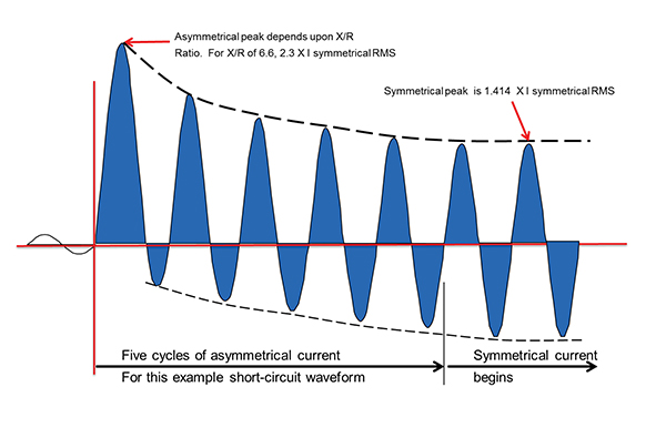
Figure 1 illustrates the two extreme conditions of short-circuit current behavior in a normal low-voltage circuit. The terms symmetrical and asymmetrical are used to describe the symmetry of the waveform about the horizontal zero axis. The asymmetrical waveform has a first half cycle at a higher amplitude than the second half cycle, hence an asymmetry about the x-axis. This first half cycle presents the highest peak current during a short-circuit, the peak of which depends upon the X/R ratio of the circuit at the time of the short-circuit. The X/R ratio discussion will be left for another day. This asymmetrical waveform is what the power distribution system would experience without an overcurrent protective device. As shown in this image, the first few cycles during a short-circuit event are asymmetrical but, if left to persist, eventually become symmetrical. Remember, there are power circuit breakers that can hold their contacts closed for upwards of 30 cycles. The reason for the decay of the waveform from one that is asymmetrical to one that is symmetrical pertains to the contribution factors to the short-circuit current. Short-circuit contributors are generators and motors. These contributors are not there all the time; they decay away. For example, when you collapse the voltage on a motor driving a load, the inertia of the load will continue to spin the rotor of the motor, which then through back EMF generates current in the stator, basically turning the motor into a generator. But that inertia won’t last forever, it eventually slows down and goes away. This is a very basic explanation but, I think, it is an effective way of explaining the decay of asymmetrical current to symmetrical current. It is much more complex than that, but I trust you get the point.
As noted above, the Peak value will vary depending upon the X/R ratio of the system. For an X/R ratio of 6.6 (15% power factor), the peak value is 2.3 times the symmetrical RMS current. As the X/R ratio decreases, the peak current value will also decrease. For example, for an X/R ratio of 1.98 (45% PF), the peak current is 1.75 times the symmetrical RMS current. The worst-case scenario, and the scenario that let-through curves are based on, is a system with 15% power factor or 6.6 X/R ratio during the short-circuit event.
The peak current shown in the figure above is an important data point. Magnetic forces on the power distribution system will vary as the square of the peak current and thermal energy varies as the square of the RMS current.
To illustrate the power that magnetic forces inflict on the power distribution system during the first cycle of a short-circuit current, a video demonstration of a 2/0 conductor experiencing 1 cycle of short-circuit current is quite revealing. The video shows 1 cycle of 26,000 amps flowing through 90 ft of 2/0 conductor. The peak let-through for this example proved to be 48,100 A. The clearing time was 0. 0167 seconds. (1 cycle = 0.016 seconds.)
Now that we have a taste of what the waveform looks like during a fault, as well as what that translates to in practical application, let’s explore some more details around current limitation and the let-through charts.
Peak Let-Through Current and Clearing Time
UL 248, Low-voltage Fuses, is the standard and is separated into various parts that address the various classes of fuses that exist. I’ll focus on part 8, to keep it simple, which addresses the Class J fuse. I am picking the fuse for this discussion as when it comes to current limitation, the fuse shines. You may have heard me ask this question in some of my training seminars on overcurrent protection but I’ll ask it again: “Do you know what a fuse eats for breakfast, lunch, and dinner and never gains weight?” The answer to that question is “current.” These devices love amps. The more, the better and they eat ’em up. I think you’ll see what I mean as we talk about current limitation and the let-thru curves.
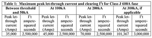
UL standards provide the performance criteria that listed solutions must pass to earn the label. UL 248 provides the maximum peak let-through current and clearing I2t values for the various classes of fuses. Fuse designs must not exceed these values. Let’s focus on the 600A Class J fuse which has maximum peak let-through currents from UL 248 as shown in the above table:
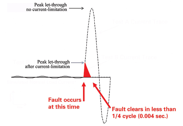
Let’s assume that the available symmetrical RMS short-circuit current is 100,000 A. The peak let- through of this current without an overcurrent protective device in the picture would be 2.3 times the 100,000 RMS amp short-circuit current or 230,000 amps. To be called a current-limiting device, one of the requirements is to limit this peak current to 45,000 amps or less (see table 1). Figure 2 is a generic image that shows the difference between peak current without current limitation and the peak let-through current due to a current-limiting device. When the peak current is limited by the fuse, the duration that the current is permitted to flow is also reduced. So, through current limitation, we reduce not only the magnetic forces but also the thermal heating that a short-circuit current causes.
This translates into much less magnetic force and less energy overall. The practical effects on the power distribution system are witnessed in a video of the same application shown previously (2/0 conductor and 26,000 amps) with a slight change in that we now have a current-limiting fuse ahead of this conductor. The current-limiting fuse reduced the peak let-through current from 48,100 to 10,200 amps. The video provides a visual illustration of the impact that the reduced magnetic forces have on the power distribution system. The conductor barely moves in this example.
Current limitation reduces the peak let-through and the duration that the current is permitted to flow. The total clearing time of the short-circuit current is less than ½ of a cycle. The two video links above illustrate the impact of current limitation versus not providing current limitation on the power distribution system.
Current-Limitation Curves
Now that we understand the short-circuit waveform and what current-limiting devices do to that waveform to reduce the mechanical and thermal stress on the power distribution system, let’s see how the published let-through curves relate to this discussion.
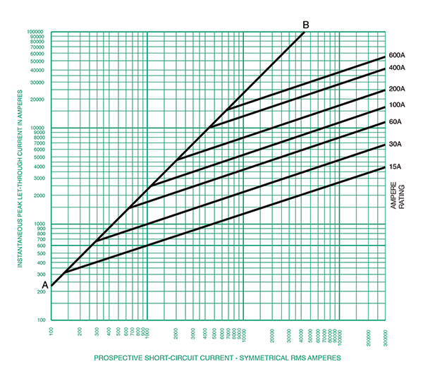
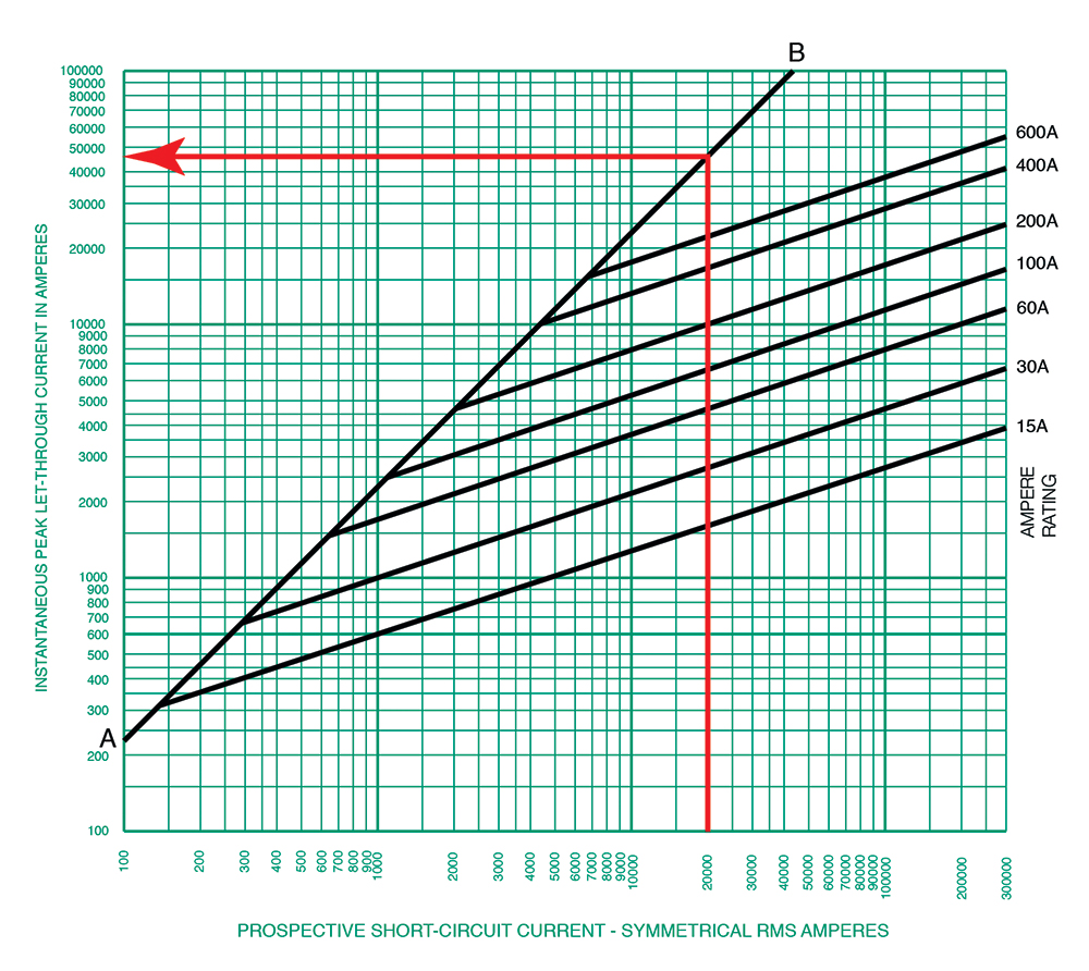
What is shown in figure 3 is the Current-Limitation curve for the Class J Dual-element Time-Delay fuse of a specific manufacturer. These curves may vary by manufacturer; always make sure the document you are reviewing relates to the product you are applying.
This curve tells us a lot of information about the waveform of the short-circuit current. In fact, it relates only to the first half cycle of that waveform. Let’s first understand the anatomy of this graph referencing figure 3. Here’s what we know.
- The horizontal axis is in symmetrical RMS amps and the vertical axis is in Peak amps.
- The AB line corresponds to a short-circuit power factor of 15% which is associated with an X/R ratio of 6.6. This will present a worst-case peak current that the device would have to interrupt. For an X/R ratio of 6.6, the equation for that linear line is
I Peak = 2.3 × I RMS
This equation enables us to calculate the peak current for any RMS short-circuit current provided that there is no current-limiting overcurrent device in the picture. As an example, for a 20,000-amp RMS symmetrical short-circuit current, the peak asymmetrical current is calculated as follows:
I Peak = 2.3 × 20,000 Amps = 46,000 Amps
For a circuit with an X/R ratio of 6.6 and 20,000 amps of RMS short-circuit current, the peak current expected is 46 kA.
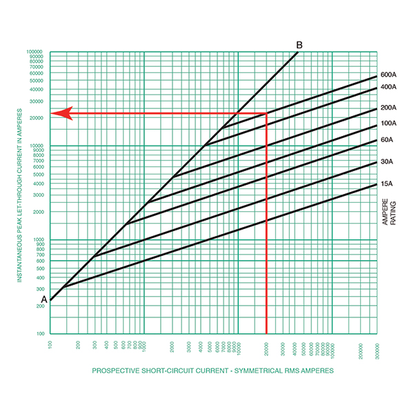
To get this from the curve, we find 20,000 amps along the horizontal and trace that up to when we hit the AB line. When we hit the AB line, we follow it to the left on the Y Axis and read the number. See figure 4 for that example.

- The other lines on this curve are those for each individual amp-rated fuse. This helps us understand the current limitation capability of the specific fuse. For our example, we were working with the 600 A fuse. To determine the peak current when applying a 600 A fuse to this circuit with an X/R ratio of 6.6 and 20,000 amps available RMS, we follow a similar process that we did in step 2 above, but instead we stop at the diagonal line for the 600 A fuse and draw a horizontal line to the vertical axis to read the reduced peak current. See figure 5 for this example where we can estimate the peak current to be 24,000 amps. This is a considerable reduction from 46 kA to 24 kA in peak current. It’s considerable when we understand that the magnetic forces are calculated as the square of the peak current. The current limiting effects of this OCPD almost cut the peak in half.
- Where the specific amp fuse curve meets the AB line is where the fuse enters its current-limiting region.
Parting Remarks
Short-circuit conditions place magnetic forces and generate heat within the power distribution system when permitted to flow. When devices operate in their current-limiting region, the stress on the system is reduced considerably. Reducing the peak current and the time a short-circuit is permitted to flow in a circuit makes it easier for the equipment to hold it together under the forces that these extreme conditions place on all the power carrying components. Proper application of electrical distribution equipment relies on our understanding of these concepts.
In this article we only talked about the peak current let-through; up and over on the curve. In my next article we’ll speak to the RMS let-through; up, over and down on the curve.
As always, keep safety at the top of your list and ensure you and those around you live to see another day.