
One of the most fundamental calculations made on a power distribution system is that which yields available short-circuit current. The September – October 2012 issue of IAEI magazine included an article titled “Going to Basics, Maximum Fault Current” which spoke to this topic but did not get into the math. I have received many requests ever since to get into the math. I trust this article will satisfy inquiring minds with details around calculating available fault current and provide some equations for the student to explore.
Available Short-Circuit Current
Maximum available short-circuit current is an important parameter for every power distribution system as it provides a data point necessary to ensure equipment is being applied within its rating and the system is performing to meet expectations. Available short-circuit current is used in many other applications as well.
The National Electrical Code demands this data point for enforcement of such Sections as 110.9, Interrupting Rating; 110.10 Circuit Impedance, Short-Circuit Current Ratings, and other Characteristics; and 110.24 Available Fault Current. Whether you are a designer, installer or inspector, you will at some point in your career be faced with calculating available fault current. Understanding the math behind this and how calculated short-circuit currents are used can only broaden knowledge and understanding. It may also help us realize that a qualified individual should be the one making these calculations. So for the sake understanding, I offer this article to get you on your way.
Fundamentals of Calculating Short-Circuit Current
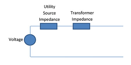
Everything you need to know about calculating fault currents, you learned in circuits 101, trigonometry, and basic math classes. Figure 1 illustrates a simple single-line diagram that very well could be your basic service entrance for a commercial or industrial installation.
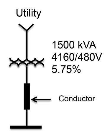
Figure 2 is the basic circuit diagram of what is represented in Figure 1 and that would be used to calculate available fault current at any point in the above simple single line diagram. Engineers will call that which you see in Figure 2 an impedance diagram as it basically converts each component in the Figure 1 above into impedance values. For those of you who are up on circuits 101, what you see below, when all impedances are added together, is a “Thevanin Equivalent” circuit which includes an impedance and a voltage source. This basic circuit will be used throughout this article.
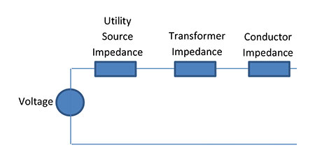
Assumptions will have to be made for calculations and to simplify our work for this document.
The assumptions for the transformer that will be used as part of the example for this article will include that which follows. This information should be available when reading the nameplate of the transformer.
Transformer kVA 1500
Primary Voltage 4,160 V
Secondary Voltage 480 V
% Impedance 5.75%
The assumption is for the utility available short-circuit current. For this exercise 50,000 amps will be used. Before a study is conducted, the utility is contacted to obtain this information. They may provide the available fault current in one of a few different ways. The most straightforward and probably most seen data from the utility will be an available fault current in kA. Some utilities may provide the data as short-circuit MVA instead. This article will provide equations to accommodate both forms of input but cater to a utility available short-circuit current of 50 kA.
With regard to conductor impedance, the following calculations will ignore the resistance of the conductor and only use the reactance. This will do two things for the sake of this article. First, it will result in a higher fault current than would be calculated had we taken into consideration both the resistance and reactance. Second, it will keep the math simple. A final section of this article will provide analysis results that include the resistance and reactance of the conductors and the utility. The methods used mirror those used by such software programs as SKM Systems Analysis A-Fault.
This article will also assume no motor contribution. Maximum available short-circuit current should include all short-circuit contributors. We are not including this contribution for this effort for simplicity sake.
Basic Transformer Calculations
The very first step of this process is the calculation of full-load amps (FLA) for the transformer. Yet another basic calculation that an electrical professional will have to perform at some point in their career and that some perform many times a day. The equations for calculating FLA are included below:
| FLA Secondary | = kVA |
| (√3)×(kVsec) |
| FLA Secondary | = 1500 |
| [(√3)×(0.480)] =1,804 Amps |
This 1500 kVA transformer has a secondary FLA of 1,804 amps. This parameter is necessary to select the secondary conductors for this transformer. Based on this FLA and the use of Table 310.15(B)(16) from NEC 2014, the conductors used on the secondary of the transformer will be a quantity of 5-500 MCM conductors per phase.
Calculating Short-Circuit Current On Secondary of Main Transformer
There are two ways to approach calculating the available fault current at the secondary of a transformer. We can calculate the maximum amount that the transformer will let through, as if the power generation facility was hooked directly to the line side of the transformer, or we can calculate the available fault current considering the provided available fault current from the utility. The former approach which results in the maximum amount of fault current that a transformer will let through is referred to as an “infinite bus” calculation. The circuit of figure 2 can be re-drawn to include zero impedance for the utility which will reduce the overall impedance of the circuit and so increase the value of calculated short-circuit current. Figure 3 will yield the maximum available fault current that a transformer can supply.
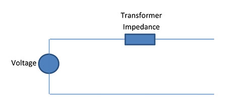
Figure 3 only includes the impedance of the transformer. The equation to calculate the maximum available fault current that a transformer can supply is as follows:
| Isc | = (Transformer kVA) × 100 |
| (√3)×(Secondary kV)×(%Z transformer) |
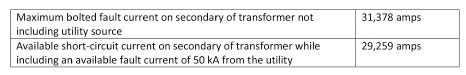
Using the information stated above for the example 1500 kVA transformer for this example, the maximum available fault current that this specific transformer will let through is 31,378 amps and is calculated as follows:
| Isc | = 1500 × 100 |
| (√3)×(0.480)×(5.75) = 31,378 amps |
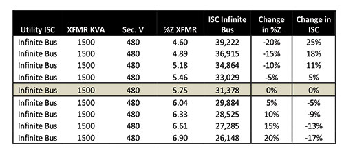
What this tells us is that the secondary of the transformer cannot see any more fault current than what we have calculated. There are NO changes on the utility side that can impact this available fault current to a point where it would be greater than 31,378 amps. The only way this service would see more than 31,378 amps would be if we changed the transformer and the new transformer which would presumably be the same in all other characteristics, has a different % impedance. Figure 4 is a table that includes the results of varying the impedance of the subject transformer +/- 20% in increments of 5% as compared with the 5.75% impedance value used in this example. This illustrates how a change in transformer impedance will impact the maximum available fault current that it can let through.
As illustrated in figure 4, changing a transformer and varying its impedance can have a significant impact on the system. If I were to hazard a guess, I would say that in most cases, a utility changing the service-entrance transformer would be recognized by the facility. The challenge would be for the facility owner or resident employees to understand how that change may impact their power distribution system. When changes are made, labels like that included in Section 110.24 of the NEC, should be updated.
This calculation does not consider the source impedance of the utility and nor does it include any load-side conductors. Let’s next explore the impact of adding in the utility available fault current.
Calculating Short-Circuit Current Including Utility Available Fault Current
As in most situations, we take conservative shortcuts, conservative on the side of safety, until situations present themselves that warrant digging into the details. The above shortcut for calculating fault current is conservative, in that it did NOT consider the utility available fault current yielding a maximum value. When considering interrupting and other similar ratings, devices and equipment that can accommodate this conservative value of fault current need no further investigation. When new or existing equipment cannot handle this conservatively high available fault current, further detailed analysis could be conducted or the equipment could be replaced or sized appropriately. The following will consider adding utility provided available fault current. Specifically, 50 kA available from the utility. This will illustrate that the calculated 31,378 amps could be reduced by doing so.
Below, are two equations that address when kA is available and when Short-Circuit MVA is available. For this example, we will use the equation below that assumes the utility has provided you with an available fault current in kA.
The circuit diagram now looks like that shown in figure 5.
The first step required is to convert the utility provided available fault current information (50 kA) into a source impedance.
When kA is provided by the utility:
| %Z Utility | = KVA Transformer × 100 |
| (Isc Utility) × (√3) × (kV Primary) |
When Short-Circuit MVA is provided by the Utility:
| %Z Utility | = KVA Transformer |
| Short – Circuit kVA of Utility System |
For a given utility available fault current of 50 kA, the %Z of the utility is calculated as follows
| %Z Utility | = 1500 × 100 |
| (50,000) × (√3) × (4.160) = 0.420 |
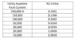
Figure 6 provides utility source impedance values for varying utility available fault currents for this specific example. As noted above, the transformer kVA and primary voltage will play a key role in these values.
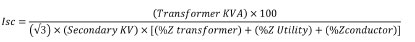
The equation for calculating the available fault current at the secondary of the transformer which includes the impedance of the utility is as follows:
| Isc | = (Transformer KVA) × 100) |
| (√3) × (Secondary KV) × [(%Ztransformer)+(%Z Utility)] |
Inserting all of the known variables, the new available fault current is calculated as follows:
| Isc | = 1500 × 100 |
| (√3)×(0.480)× [(5.75)+(0.4164)] = 29,259 Amps |
If we compare the infinite bus calculation and that which included the source impedance of the utility (available fault current of 50,000 amps) we see that the available short-circuit current dropped from 31,378 amps to 29,259 amps, a 6.8% reduction in available fault current (2,119 amps).
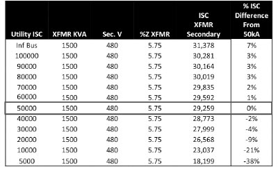
The impact of a varying utility available fault current is illustrated in figure 7. This table shows how the calculated available short-circuit current varies for changing utility source fault current values. The 50 kA utility available fault current is used as the value to which changes are compared. It is interesting to see that increasing the available fault current from the utility, assuming a starting point of 50 kA, doesn’t have as great of an impact as one would think. For example, doubling the utility available fault current from 50 kA to 100 kA only increases the transformer secondary available fault current by 3%, or 1,022 amps. For most overcurrent protective device application, this change should not be significant. I have heard some say we should not label the service-entrance equipment because the utility could make switching changes on the line side which would impact the number on the label. Figure 7 is a good example that shows that even if an infinite bus was not used, changes on the utility side do not have as significant of an impact on the short-circuit current as one would think.
Just to recap where we are in this discussion, the available fault currents are as in figure 7a.
The next thing we have to consider is the conductor on the secondary of the transformer. This will reduce the available fault current even further.
Calculating – After Length of Conductor
Conductors can have a considerable impact on available fault current. Let’s continue the analysis of this 1500 kVA transformer example adding parallel 500MCM conductors on its load side.
The equivalent circuit has already been provided as part of figure 1. Now let’s review the impact of conductor length on available fault current. We need the following equation:

The data needed for this example is retrieved from the National Electrical Code. From Table 9 of NEC 2014 for a 500 MCM conductor in steel conduit, the Xl (reactance) is found to be 0.048 Ohms/1000ft. For this example, as stated earlier, we are only using the reactance value which will result in slightly higher short-circuit current values and make the math for this publication more palatable. For a 1500 kVA transformer with 1,804 full load amps, we will need 5- 500MCM conductors in parallel per phase. The calculation is made as follows:

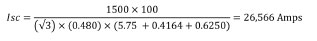
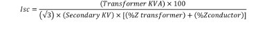
the equation to calculate the available fault current is as follows:
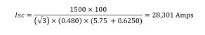
Putting in all of the known variables, we calculated the ISC as follows:
The same calculation assuming an infinite bus, removing the utility impedance, is as follows:
To summarize again,
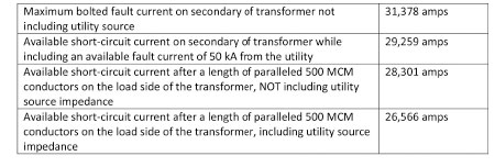
As can be seen here, including more details reduces the available fault current. In this case the fault current was reduced from 31,378 amps to 26,566 amps, approximately 15.3%.
Final Calibration
So we have walked through the calculation of available fault current for service-entrance equipment. We showed how shortcuts result in conservative available short-circuit currents which, for the purpose of evaluating interrupting ratings and / or SCCR ratings, provide a safety factor for the design. We also showed how reducing available fault currents through a more detailed analysis can be achieved but takes more effort and expertise. Let’s look at the above example with an eye on other tools that may be available.
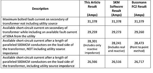
There are various tools at our disposal when we consider calculating available fault current. Some are quite expensive and take trained specialists to use. Those would include such software applications as SKM Systems Analysis tools. These applications are indeed quite thorough and produce very detailed reports. There are also tools that are free such as the Eaton Bussmann FC2 short-circuit calculator. Figure 8 summarizes what we accomplished above AND provides a comparison with SKM and with the Bussmann FC2 application. The Bussmann FC2 calculator is free and available on the web or for any IPHONE or ANDROID via either products App Store. Visit www.cooperbussmann.com/fc2 for more information. You will note that the SKM software result leverages both the real and reactive component of the conductor. The impedance values were taken straight from Table 9 in NEC 2014 for copper conductors in steel conduit.
Again, none of the examples shown above and included in this article considers motor contribution. This was an exercise meant to provide some background to the discussion of short-circuit currents and so simplicity was our friend. Motor contribution can be very important for these calculations. From a math and/or system circuit perspective, when you include motor contribution the impedance is in parallel with the utility source impedance, transformer impedance and the conductor impedance. This acts to reduce the overall impedance in the circuit of figure 2 and hence increasing the calculated short-circuit current. The reset is left to the student. (I’ve always wanted to say that.)
Closing Remarks
Available fault current is a very important parameter to consider in your design, installation and inspection. Tools are available on the market that help calculate available short-circuit current. Leverage these resources to meet NEC and product application requirements.
As always, keep safety at the top of your list and ensure you and those around you live to see another day.